Chapter 10 Type 2 & 3 Gauge r&R Study
10.1 Type 2 Gauge r&R Study
The example data are taken from Houf & Berman (1988) and concern the thermal impedance of \(10\) different power modules (in \(^\circ\)C per \(\text{Watt} \times 100\)) as measured by \(3\) different operators. Each operator measured each part \(3\) times:
| Part | Operator | Measurement |
|---|---|---|
| 1 | A | 37 |
| 1 | A | 38 |
| 1 | A | 37 |
| 1 | B | 41 |
| 1 | B | 41 |
| 1 | B | 40 |
| 1 | C | 41 |
| 1 | C | 42 |
| 1 | C | 41 |
| 2 | A | 42 |
| 2 | A | 41 |
| 2 | A | 43 |
| 2 | B | 42 |
| 2 | B | 42 |
| 2 | B | 42 |
| 2 | C | 43 |
| 2 | C | 42 |
| 2 | C | 43 |
| 3 | A | 30 |
| 3 | A | 31 |
| 3 | A | 31 |
| 3 | B | 31 |
| 3 | B | 31 |
| 3 | B | 31 |
| 3 | C | 29 |
| 3 | C | 30 |
| 3 | C | 28 |
| 4 | A | 42 |
| 4 | A | 43 |
| 4 | A | 42 |
| 4 | B | 43 |
| 4 | B | 43 |
| 4 | B | 43 |
| 4 | C | 42 |
| 4 | C | 42 |
| 4 | C | 42 |
| 5 | A | 28 |
| 5 | A | 30 |
| 5 | A | 29 |
| 5 | B | 29 |
| 5 | B | 30 |
| 5 | B | 29 |
| 5 | C | 31 |
| 5 | C | 29 |
| 5 | C | 29 |
| 6 | A | 42 |
| 6 | A | 42 |
| 6 | A | 43 |
| 6 | B | 45 |
| 6 | B | 45 |
| 6 | B | 45 |
| 6 | C | 44 |
| 6 | C | 46 |
| 6 | C | 45 |
| 7 | A | 25 |
| 7 | A | 26 |
| 7 | A | 27 |
| 7 | B | 28 |
| 7 | B | 28 |
| 7 | B | 30 |
| 7 | C | 29 |
| 7 | C | 27 |
| 7 | C | 27 |
| 8 | A | 40 |
| 8 | A | 40 |
| 8 | A | 40 |
| 8 | B | 43 |
| 8 | B | 42 |
| 8 | B | 42 |
| 8 | C | 43 |
| 8 | C | 43 |
| 8 | C | 41 |
| 9 | A | 25 |
| 9 | A | 25 |
| 9 | A | 25 |
| 9 | B | 27 |
| 9 | B | 29 |
| 9 | B | 28 |
| 9 | C | 26 |
| 9 | C | 26 |
| 9 | C | 26 |
| 10 | A | 35 |
| 10 | A | 34 |
| 10 | A | 34 |
| 10 | B | 35 |
| 10 | B | 35 |
| 10 | B | 34 |
| 10 | C | 35 |
| 10 | C | 34 |
| 10 | C | 35 |
10.1.1 Results Overview
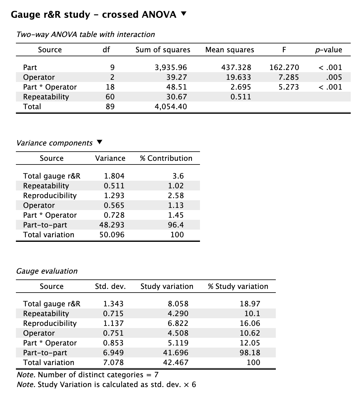
10.1.1.1 Variance Components
| JASP | By Hand | JMP | Minitab | R | |
|---|---|---|---|---|---|
| Total Gage R&R | 1.804 | 1.804 | 1.804 | 1.804 | 1.804 |
| Repeatability | 0.511 | 0.511 | 0.511 | 0.511 | 0.511 |
| Reproducibility | 1.293 | 1.293 | 1.293 | 1.293 | 1.293 |
| Operator | 0.565 | 0.565 | 0.565 | 0.565 | 0.565 |
| Part:Operator | 0.728 | 0.728 | 0.728 | 0.728 | 0.728 |
| Part-To-Part | 48.293 | 48.293 | 48.293 | 48.293 | 48.293 |
| Total Variation | 50.096 | 50.096 | 50.096 | 50.096 | 50.096 |
10.1.1.2 % Contribution
| JASP | By Hand | JMP | Minitab | R | |
|---|---|---|---|---|---|
| Total Gage R&R | 3.60 | 3.60 | 3.60 | 3.60 | 3.60 |
| Repeatability | 1.02 | 1.02 | 1.02 | 1.02 | 1.02 |
| Reproducibility | 2.58 | 2.58 | 2.58 | 2.58 | 2.58 |
| Operator | 1.13 | 1.13 | 1.13 | 1.13 | 1.13 |
| Part:Operator | 1.45 | 1.45 | 1.45 | 1.45 | 1.45 |
| Part-To-Part | 96.40 | 96.40 | 96.40 | 96.40 | 96.40 |
| Total Variation | 100.00 | 100.00 | 100.00 | 100.00 | 100.00 |
10.1.3 By Hand
# number of levels
o <- nlevels(dat$Operator)
p <- nlevels(dat$Part)
n <- length(dat$Measurement) / (o * p)

# totals
grand_total <- sum(dat$Measurement)
C <- grand_total^2 / (o * p * n)

cell_totals <- with(dat, tapply(Measurement, list(Operator, Part), sum))
row_totals  <- rowSums(cell_totals)
col_totals  <- colSums(cell_totals)

# SS total
SS_total <- sum(dat$Measurement^2) - C

# SS O (Operator)
SS_O <- sum(row_totals^2) / (p * n) - C

# SS P (Part)
SS_P <- sum(col_totals^2) / (o * n) - C

# SS O×P
SS_OP <- sum(cell_totals^2) / n - SS_O - SS_P - C

# SS error
cell_sumsq <- with(dat, tapply(Measurement, list(Operator, Part), function(x) sum(x^2)))
SS_E <- sum(cell_sumsq - (cell_totals^2)/n)

# degrees of freedom
df_O <- o - 1
df_P <- p - 1
df_OP <- (o - 1) * (p - 1)
df_E <- o * p * (n - 1)

# mean squares
MS_O  <- SS_O / df_O
MS_P  <- SS_P / df_P
MS_OP <- SS_OP / df_OP
MS_E  <- SS_E / df_E

# Variance component estimates assuming that both Operators and Parts are random effects
sigma2_E  <- MS_E
sigma2_OP <- (MS_OP - MS_E) / n
sigma2_O  <- (MS_O - MS_OP) / (n * p)
sigma2_P  <- (MS_P - MS_OP) / (n * o)

reprod <- sigma2_O + sigma2_OP
repeatab <- sigma2_E
gauge <- reprod + repeatab
total <- gauge + sigma2_P

varComp <- c(gauge, repeatab, reprod, sigma2_O, sigma2_OP, sigma2_P, total)

# %Contribution
percContrib <- varComp / total * 100

res <- matrix(c(varComp, percContrib),
              nrow = 7, ncol = 2, byrow = FALSE)

colnames(res) <- c("Variance Components", "% Contribution")

rownames(res) <- c("Total Gage R&R", "Repeatability", "Reproducibility", "Operator",
                   "Part:Operator", "Part-To-Part", "Total Variation")

res
## Variance Components % Contribution
## Total Gage R&R 1.8037037 3.600473
## Repeatability 0.5111111 1.020257
## Reproducibility 1.2925926 2.580216
## Operator 0.5646091 1.127047
## Part:Operator 0.7279835 1.453168
## Part-To-Part 48.2925926 96.399527
## Total Variation 50.0962963 100.000000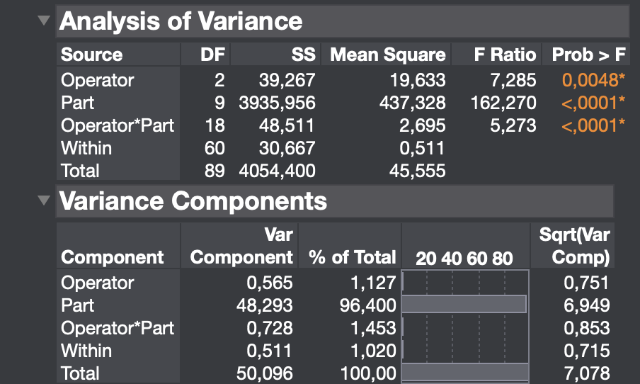
10.1.5 Minitab
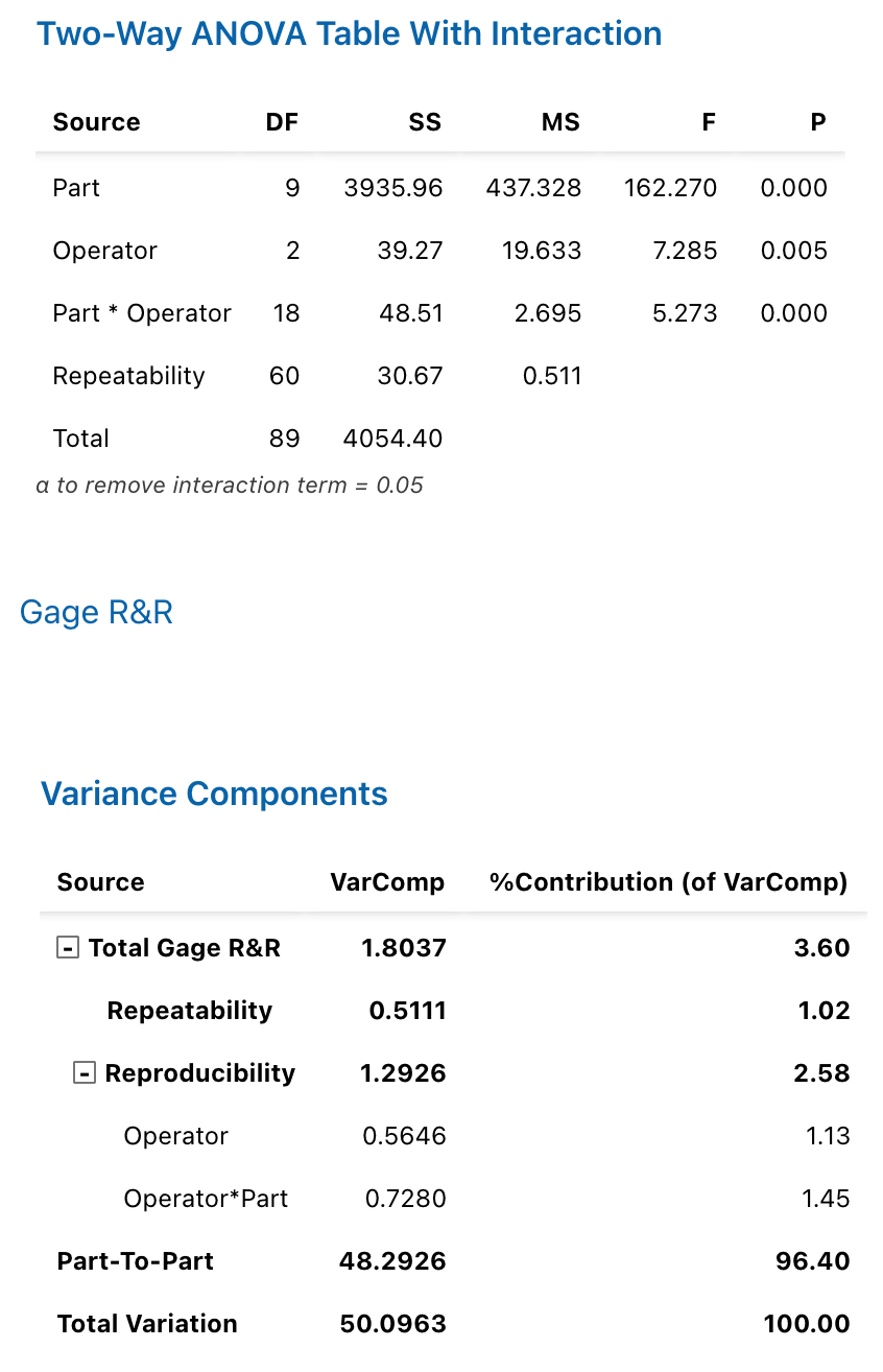
Figure 10.3: Minitab Output for Type 2 Gauge r&R Analysis (Part 1)
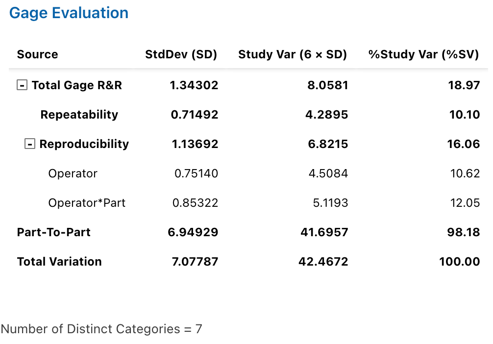
Figure 10.4: Minitab Output for Type 2 Gauge r&R Analysis (Part 2)
10.1.6 R
## Complete model (with interaction):
##
##               Df Sum Sq Mean Sq F value   Pr(>F)
## Part           9   3936   437.3 162.270 2.29e-15
## Operator       2     39    19.6   7.285  0.00481
## Part:Operator 18     49     2.7   5.273 5.06e-07
## Repeatability 60     31     0.5
## Total         89   4054
##
## alpha for removing interaction: 0.05
##
## Gage R&R
##
##                      VarComp %Contrib
## Total Gage R&R     1.8037037     3.60
##   Repeatability    0.5111111     1.02
##   Reproducibility  1.2925926     2.58
##     Operator       0.5646091     1.13
## Part:Operator      0.7279835     1.45
## Part-To-Part      48.2925926    96.40
## Total Variation   50.0962963   100.00
##
##                      StdDev  StudyVar %StudyVar
## Total Gage R&R    1.3430204  8.058122     18.97
##   Repeatability   0.7149204  4.289522     10.10
##   Reproducibility 1.1369224  6.821535     16.06
##     Operator      0.7514047  4.508428     10.62
## Part:Operator     0.8532195  5.119317     12.05
## Part-To-Part      6.9492872 41.695723     98.18
## Total Variation   7.0778737 42.467242    100.00
##
## Number of Distinct Categories = 7
10.2 Type 3 Gauge r&R Study
Consider an example from Gadim & Doniavi (2018). The data concern the tensile strength of polymer yarns. Each of the \(30\) yarns was measured \(3\) times:
| Part | Measurement |
|---|---|
| 1 | 1.6245 |
| 1 | 1.6225 |
| 1 | 1.6278 |
| 2 | 1.7277 |
| 2 | 1.7254 |
| 2 | 1.7307 |
| 3 | 1.6847 |
| 3 | 1.6828 |
| 3 | 1.6874 |
| 4 | 1.8249 |
| 4 | 1.8226 |
| 4 | 1.8273 |
| 5 | 1.7114 |
| 5 | 1.7054 |
| 5 | 1.7160 |
| 6 | 1.8072 |
| 6 | 1.8006 |
| 6 | 1.8160 |
| 7 | 1.7681 |
| 7 | 1.7590 |
| 7 | 1.7677 |
| 8 | 1.8650 |
| 8 | 1.8561 |
| 8 | 1.8737 |
| 9 | 1.6670 |
| 9 | 1.6579 |
| 9 | 1.6700 |
| 10 | 1.8546 |
| 10 | 1.8520 |
| 10 | 1.8583 |
| 11 | 1.7948 |
| 11 | 1.7925 |
| 11 | 1.7976 |
| 12 | 1.9814 |
| 12 | 1.9799 |
| 12 | 1.9846 |
| 13 | 1.9046 |
| 13 | 1.9022 |
| 13 | 1.9081 |
| 14 | 2.0546 |
| 14 | 2.0520 |
| 14 | 2.0583 |
| 15 | 1.9654 |
| 15 | 1.9594 |
| 15 | 1.9700 |
| 16 | 2.1570 |
| 16 | 2.1479 |
| 16 | 2.1600 |
| 17 | 1.8684 |
| 17 | 1.8624 |
| 17 | 1.8730 |
| 18 | 2.0548 |
| 18 | 2.0526 |
| 18 | 2.0575 |
| 19 | 1.8109 |
| 19 | 1.8084 |
| 19 | 1.8135 |
| 20 | 1.8896 |
| 20 | 1.8812 |
| 20 | 1.8901 |
| 21 | 1.8840 |
| 21 | 1.8749 |
| 21 | 1.8870 |
| 22 | 1.9694 |
| 22 | 1.9634 |
| 22 | 1.9740 |
| 23 | 1.7645 |
| 23 | 1.7629 |
| 23 | 1.7675 |
| 24 | 1.9130 |
| 24 | 1.9039 |
| 24 | 1.9159 |
| 25 | 1.9415 |
| 25 | 1.9434 |
| 25 | 1.9500 |
| 26 | 1.8774 |
| 26 | 1.8714 |
| 26 | 1.8820 |
| 27 | 1.8737 |
| 27 | 1.8713 |
| 27 | 1.8769 |
| 28 | 1.9076 |
| 28 | 1.8992 |
| 28 | 1.9081 |
| 29 | 1.9550 |
| 29 | 1.9461 |
| 29 | 1.9637 |
| 30 | 1.9046 |
| 30 | 1.9022 |
| 30 | 1.9081 |
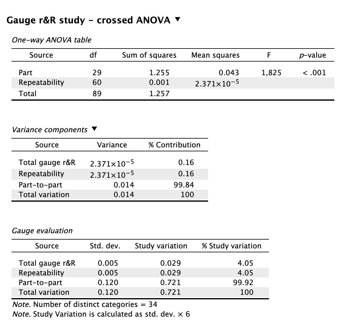
10.2.1 Results Overview
10.2.1.1 Variance Components
| JASP | By Hand | JMP | Minitab | R | |
|---|---|---|---|---|---|
| Total Gage R&R | 2.37e-05 | 2.37e-05 | 0.00002 | 2.37e-05 | 2.37e-05 |
| Repeatability | 2.37e-05 | 2.37e-05 | 0.00002 | 2.37e-05 | 2.37e-05 |
| Part-To-Part | 1.40e-02 | 1.40e-02 | 0.01400 | 1.40e-02 | 1.40e-02 |
| Total Variation | 1.40e-02 | 1.40e-02 | 0.01400 | 1.40e-02 | 1.40e-02 |
10.2.3 By Hand
# number of levels
p <- nlevels(datType3$Part)
n <- length(datType3$Measurement)
r <-  n / p

# totals
grand_total <- sum(datType3$Measurement)

# SS total
SS_total <- sum((datType3$Measurement - mean(datType3$Measurement))^2)

# SS part
partMeans <- tapply(datType3$Measurement, datType3$Part, mean)
SS_P <- sum((partMeans - mean(datType3$Measurement))^2) * r

# SS error
deviations <- datType3$Measurement - rep(partMeans, each = r)
SS_E <- sum(deviations^2)

# degrees of freedom
df_P <- p - 1
df_E <- n - p

# mean squares
MS_P  <- SS_P / df_P
MS_E  <- SS_E / df_E

# Variance components
sigma2_E <- MS_E
sigma2_P <- (MS_P - MS_E) / r

repeatab <- sigma2_E
gauge <- repeatab
total <- gauge + sigma2_P

varComp <- c(gauge, repeatab, sigma2_P, total)

# %Contribution
percContrib <- varComp / total * 100

res <- matrix(c(varComp, percContrib),
              nrow = 4, ncol = 2, byrow = FALSE)

colnames(res) <- c("Variance Components", "% Contribution")

rownames(res) <- c("Total Gage R&R", "Repeatability", "Part-To-Part", "Total Variation")

res
## Variance Components % Contribution
## Total Gage R&R 0.000023714 0.1641736
## Repeatability 0.000023714 0.1641736
## Part-To-Part 0.014420756 99.8358264
## Total Variation 0.014444470 100.0000000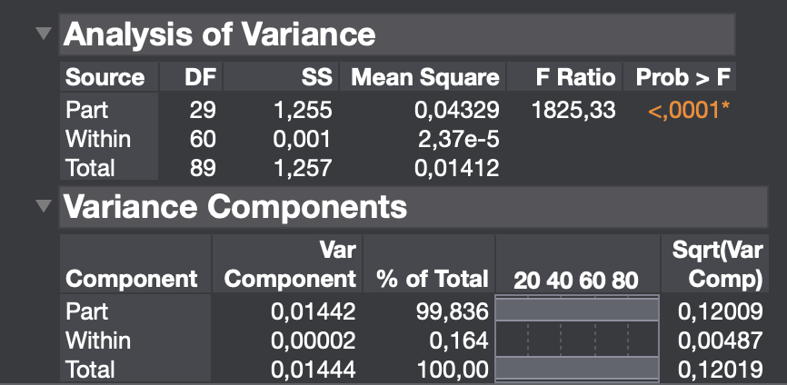
10.2.5 Minitab
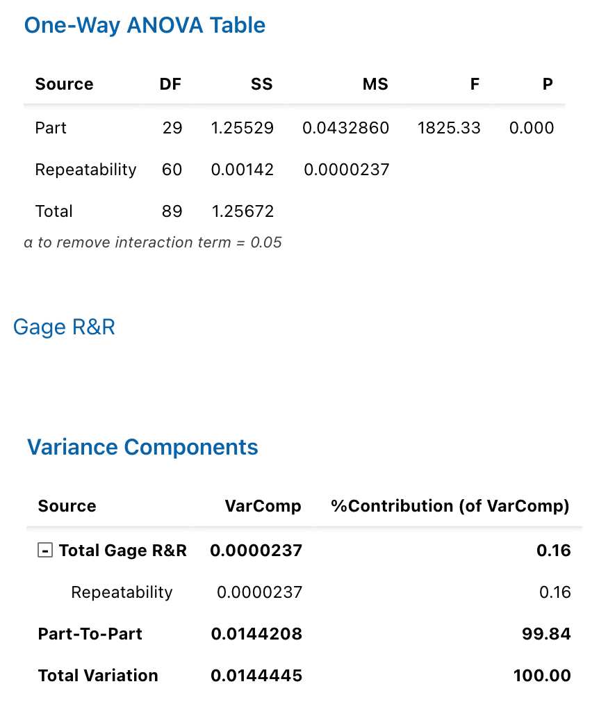
Figure 10.7: Minitab Output for Type 3 Gauge r&R Analysis (Part 1)
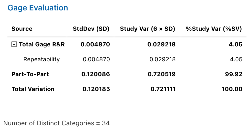
Figure 10.8: Minitab Output for Type 3 Gauge r&R Analysis (Part 2)
10.2.6 R
datType3$Operator <- rep(1, nrow(dat)) # as input for ss.rr() function
ss.rr(Measurement, Part, Operator, data = datType3, print_plot = FALSE)
## One-way ANOVA (single appraiser):
##
## Df Sum Sq Mean Sq F value Pr(>F)
## Part 29 1.2553 0.04329 1825 <2e-16
## Repeatability 60 0.0014 0.00002
## Total 89 1.2567
##
## Gage R&R
##
## VarComp %Contrib
## Total Gage R&R 0.000023714 0.16
## Repeatability 0.000023714 0.16
## Part-To-Part 0.014420756 99.84
## Total Variation 0.014444470 100.00
##
## StdDev StudyVar %StudyVar
## Total Gage R&R 0.004869702 0.02921821 4.05
## Repeatability 0.004869702 0.02921821 4.05
## Part-To-Part 0.120086453 0.72051872 99.92
## Total Variation 0.120185150 0.72111090 100.00
##
## Number of Distinct Categories = 3410.2.7 Remarks
Variance components have been estimated using expected mean squares based on ANOVA in every software.
10.2.8 References
Gadim, H. G., & Doniavi, A. (2018). Improving structural properties of polymer fibers to design and construct fiber spinneret and optimize process parameters using response surface method and gage R&R. Journal of Mechanical Science and Technology, 32(3), 1135–1142. https://doi.org/10.1007/s12206-018-0216-7
Houf, R. E., & Berman, D. B. (1988). Statistical analysis of power module thermal test equipment performance. IEEE Transactions on Components, Hybrids, and Manufacturing Technology, 11(4), 516–520. https://doi.org/10.1109/33.16692