Chapter 7 Frequencies
7.1 Binomial Test
7.1.1 Example
An example from Hays (1974, pp. 190-192):
“Think of a hypothetical study of this question: ‘If a human is subjected to a stimulus below his threshold of conscious awareness, can his behavior somehow still be influenced by the presence of the stimulus?’ The experimental task is as follows: the subject is seated in a room in front of a square screen divided into four equal parts. He is instructed that his task is to guess in which part of the screen a small, very faint, spot of light is thrown.”
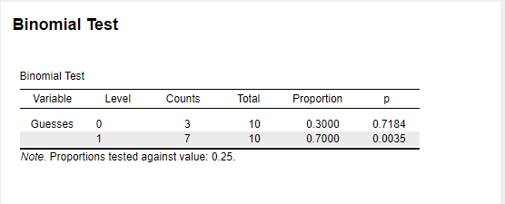
Under the null hypothesis H0, the number of correct guesses is expected to be 1/4 of the trials N. The alternative hypothesis H1 is that the number of correct guesses is larger than 1/4 of the trials N.
The subject obtained 7 correct guesses T out of 10 trials N.
What is the p-value of this result under H0?
p = 0.25
N = 10
T = 7
7.1.2 Results Overview
| By Hand | JASP | SPSS | SAS | Minitab | R | |
|---|---|---|---|---|---|---|
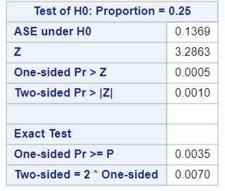
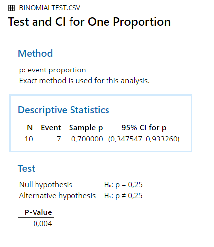
| P | 0.0035 | 0.0035 | 0.004 | 0.0035 | 0.004 | 0.0035 |
7.1.5 SPSS
DATASET NAME DataSet1 WINDOW=FRONT.
*Nonparametric Tests: One Sample.
NPTESTS
  /ONESAMPLE TEST (Guesses) BINOMIAL(TESTVALUE=0.25 SUCCESSCATEGORICAL=FIRST SUCCESSCONTINUOUS=CUTPOINT(MIDPOINT))
  /MISSING SCOPE=ANALYSIS USERMISSING=EXCLUDE
  /CRITERIA ALPHA=0.05 CILEVEL=95.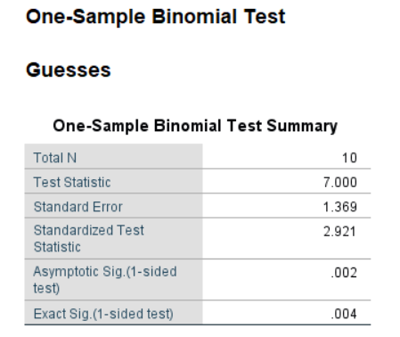
Figure 7.2: SPSS Output for Binomial Test
7.1.8 R
##
##  Exact binomial test
##
## data:  7 and 10
## number of successes = 7, number of trials = 10, p-value = 0.003506
## alternative hypothesis: true probability of success is greater than 0.25
## 95 percent confidence interval:
##  0.3933758 1.0000000
## sample estimates:
## probability of success
## 0.77.2 Multinomial Test / Chi-square Goodness of Fit Test
7.2.1 Example
Think of colored marbles mixed together in a box, where the following probability distribution holds:
| Color | p |
|---|---|
| Black | 0.4 |
| Red | 0.3 |
| White | 0.3 |
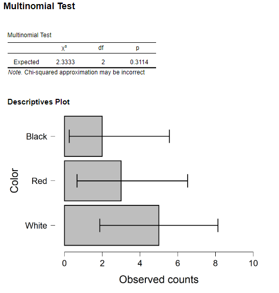
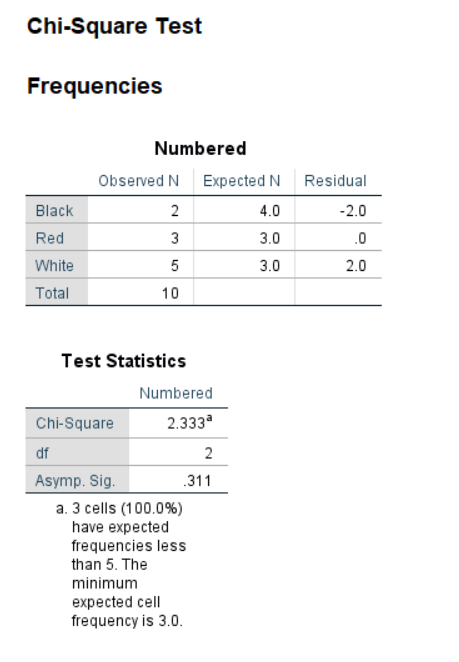
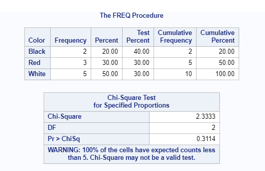
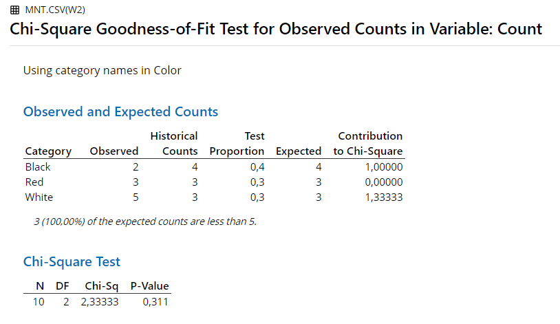
Now suppose that 10 marbles were drawn at random and with replacement. The samples shows 2 black, 3 red, and 5 white.
| Color | Count | Expected |
|---|---|---|
| Black | 2 | 4 |
| Red | 3 | 3 |
| White | 5 | 3 |
7.2.2 Results Overview
| JASP | SPSS | SAS | Minitab | R | |
|---|---|---|---|---|---|
| \(\chi ^2\) | 2.333 | 2.333 | 2.333 | 2.333 | 2.333 |
7.3 Chi-Squared-Test
An example from Hays (1974, pp. 728-731):
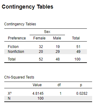
“For example, suppose that a random sample of 1– school children is drawn. Each child is classified in two ways: the first attribute is the sex of the child, with two possible categories: [Male, Female]. The second attribute […] is the stated preference of a child for two kinds of reading materials: [Fiction, Nonfiction]. […] The data might, for example, turn out to be:”
| Male | Female | |
|---|---|---|
| Fiction | 19 | 32 |
| Nonfiction | 29 | 20 |
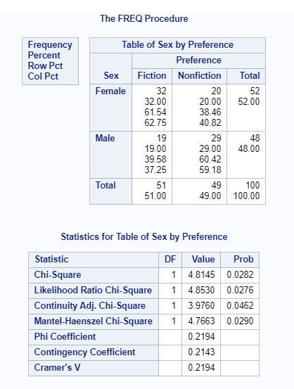
7.3.1 Results Overview
| By Hand | JASP | SPSS | SAS | Minitab | R | |
|---|---|---|---|---|---|---|
| \(\chi ^2\) | 4.83 | 4.8145 | 4.814 | 4.8145 | 4.814 | 4.8145 |
7.3.2 By Hand
Calculations by hand can be found in Hays, 1974, pp. 728-731.
Result: \(\chi ^2\) = 4.83
Significant for \(\alpha\) = .05 or less
7.3.4 SPSS
CROSSTABS
  /TABLES=Sex BY Preference
  /FORMAT=AVALUE TABLES
  /STATISTICS=CHISQ
  /CELLS=COUNT
  /COUNT ROUND CELL.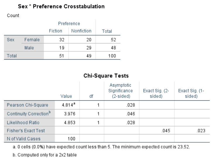
Figure 7.10: SPSS Output for Chi-Squared-Test
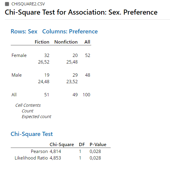
7.3.7 R
##
##  Pearson's Chi-squared test
##
## data:  chiSquare.data
## X-squared = 4.8145, df = 1, p-value = 0.02822