Chapter 6 Regression
6.1 Correlation
An example from Hays (1974, pp. 633-635):
“The teacher collected data for a class of 91 students, obtaining for each a score X, based on the number of courses in high-school mathematics, and a score Y, the actual score on the final examination for the course.”
| X | Y |
|---|---|
| 2.0 | 22 |
| 2.0 | 17 |
| 2.0 | 16 |
| 2.0 | 14 |
| 2.0 | 10 |
| 2.0 | 9 |
| 2.0 | 7 |
| 2.0 | 5 |
| 2.0 | 3 |
| 2.0 | 2 |
| 2.5 | 26 |
| 2.5 | 23 |
| 2.5 | 18 |
| 2.5 | 18 |
| 2.5 | 16 |
| 2.5 | 13 |
| 2.5 | 12 |
| 2.5 | 10 |
| 2.5 | 10 |
| 2.5 | 7 |
| 2.5 | 6 |
| 3.0 | 29 |
| 3.0 | 26 |
| 3.0 | 26 |
| 3.0 | 24 |
| 3.0 | 24 |
| 3.0 | 23 |
| 3.0 | 22 |
| 3.0 | 16 |
| 3.0 | 9 |
| 3.0 | 8 |
| 3.5 | 34 |
| 3.5 | 26 |
| 3.5 | 25 |
| 3.5 | 23 |
| 3.5 | 23 |
| 3.5 | 22 |
| 3.5 | 22 |
| 3.5 | 19 |
| 3.5 | 18 |
| 3.5 | 17 |
| 3.5 | 17 |
| 3.5 | 17 |
| 3.5 | 12 |
| 3.5 | 8 |
| 4.0 | 36 |
| 4.0 | 35 |
| 4.0 | 30 |
| 4.0 | 27 |
| 4.0 | 25 |
| 4.0 | 25 |
| 4.0 | 24 |
| 4.0 | 21 |
| 4.0 | 20 |
| 4.0 | 19 |
| 4.0 | 19 |
| 4.0 | 18 |
| 4.0 | 18 |
| 4.0 | 12 |
| 4.0 | 3 |
| 4.5 | 28 |
| 4.5 | 27 |
| 4.5 | 16 |
| 5.0 | 41 |
| 5.0 | 32 |
| 5.0 | 27 |
| 5.0 | 19 |
| 5.5 | 32 |
| 5.5 | 25 |
| 5.5 | 25 |
| 6.0 | 46 |
| 6.0 | 38 |
| 6.0 | 34 |
| 6.0 | 33 |
| 6.0 | 27 |
| 6.0 | 20 |
| 6.5 | 44 |
| 6.5 | 37 |
| 6.5 | 32 |
| 6.5 | 28 |
| 7.0 | 52 |
| 7.0 | 46 |
| 7.0 | 37 |
| 7.5 | 42 |
| 7.5 | 41 |
| 7.5 | 38 |
| 7.5 | 35 |
| 8.0 | 53 |
| 8.0 | 48 |
| 8.0 | 40 |
| 8.0 | 40 |
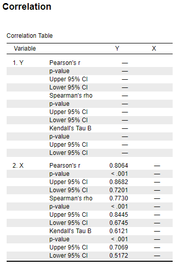
6.1.1 Results Overview
| By Hand | JASP | SPSS | SAS | Minitab | R | |
|---|---|---|---|---|---|---|
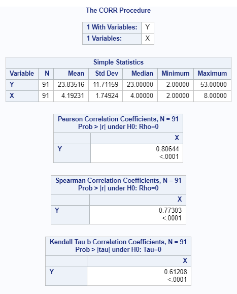
| Pearson | 0.81 | 0.8064 | 0.806 | 0.8064 | 0.806 | 0.8064 |
| Spearman | NA | 0.7730 | 0.773 | 0.7730 | 0.773 | 0.7730 |
| Kendall | NA | 0.6121 | 0.612 | 0.6120 | NA | 0.6120 |
6.1.2 By Hand
Calculations by hand can be found in Hays, 1974, pp. 633-635.
Result: r = 0.81
Note: Hays calculated only the Pearson correlation coefficient.
6.1.4 SPSS
DATASET ACTIVATE DataSet1.
CORRELATIONS
  /VARIABLES=Y X
  /PRINT=TWOTAIL NOSIG
  /MISSING=PAIRWISE.
NONPAR CORR
  /VARIABLES=Y X
  /PRINT=BOTH TWOTAIL NOSIG
  /MISSING=PAIRWISE.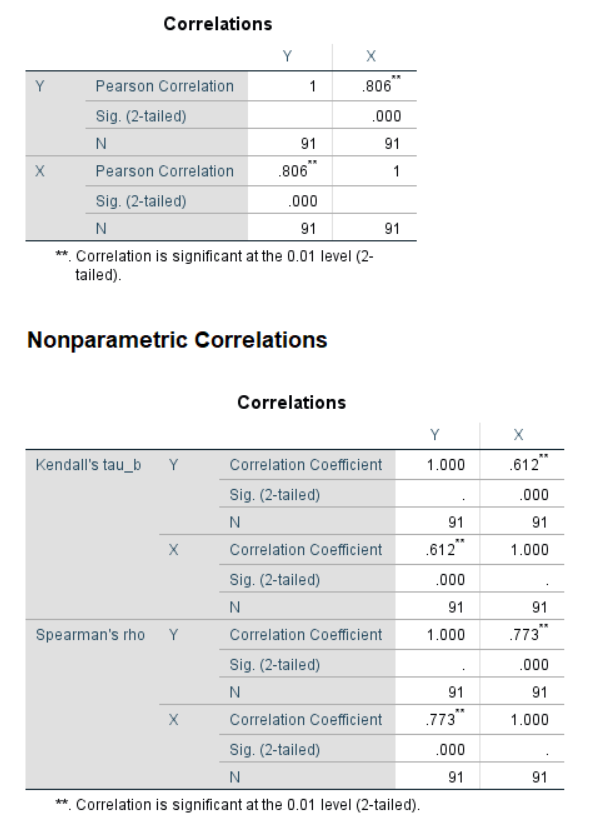
Figure 6.2: SPSS Output for Correlation
6.1.6 Minitab
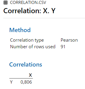
Figure 6.4: Minitab Output for Pearson Correlation
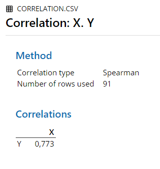
Figure 6.5: Minitab Output for Spearman Correlation
6.1.7 R
##
##  Pearson's product-moment correlation
##
## data:  corr.data$X and corr.data$Y
## t = 12.866, df = 89, p-value < 2.2e-16
## alternative hypothesis: true correlation is not equal to 0
## 95 percent confidence interval:
##  0.7200843 0.8681910
## sample estimates:
##       cor
## 0.8064365## Warning in cor.test.default(corr.data$X, corr.data$Y, method = "spearman"):
## Cannot compute exact p-value with ties##
## Spearman's rank correlation rho
##
## data: corr.data$X and corr.data$Y
## S = 28502, p-value < 2.2e-16
## alternative hypothesis: true rho is not equal to 0
## sample estimates:
## rho
## 0.7730333##
## Kendall's rank correlation tau
##
## data: corr.data$X and corr.data$Y
## z = 8.1519, p-value = 3.582e-16
## alternative hypothesis: true tau is not equal to 0
## sample estimates:
## tau
## 0.61208456.2 Linear Regression
An example from Hays (1974, pp. 633-635):
“The teacher collected data for a class of 91 students, obtaining for each a score X, based on the number of courses in high-school mathematics, and a score Y, the actual score on the final examination for the course.”
| X | Y |
|---|---|
| 2.0 | 22 |
| 2.0 | 17 |
| 2.0 | 16 |
| 2.0 | 14 |
| 2.0 | 10 |
| 2.0 | 9 |
| 2.0 | 7 |
| 2.0 | 5 |
| 2.0 | 3 |
| 2.0 | 2 |
| 2.5 | 26 |
| 2.5 | 23 |
| 2.5 | 18 |
| 2.5 | 18 |
| 2.5 | 16 |
| 2.5 | 13 |
| 2.5 | 12 |
| 2.5 | 10 |
| 2.5 | 10 |
| 2.5 | 7 |
| 2.5 | 6 |
| 3.0 | 29 |
| 3.0 | 26 |
| 3.0 | 26 |
| 3.0 | 24 |
| 3.0 | 24 |
| 3.0 | 23 |
| 3.0 | 22 |
| 3.0 | 16 |
| 3.0 | 9 |
| 3.0 | 8 |
| 3.5 | 34 |
| 3.5 | 26 |
| 3.5 | 25 |
| 3.5 | 23 |
| 3.5 | 23 |
| 3.5 | 22 |
| 3.5 | 22 |
| 3.5 | 19 |
| 3.5 | 18 |
| 3.5 | 17 |
| 3.5 | 17 |
| 3.5 | 17 |
| 3.5 | 12 |
| 3.5 | 8 |
| 4.0 | 36 |
| 4.0 | 35 |
| 4.0 | 30 |
| 4.0 | 27 |
| 4.0 | 25 |
| 4.0 | 25 |
| 4.0 | 24 |
| 4.0 | 21 |
| 4.0 | 20 |
| 4.0 | 19 |
| 4.0 | 19 |
| 4.0 | 18 |
| 4.0 | 18 |
| 4.0 | 12 |
| 4.0 | 3 |
| 4.5 | 28 |
| 4.5 | 27 |
| 4.5 | 16 |
| 5.0 | 41 |
| 5.0 | 32 |
| 5.0 | 27 |
| 5.0 | 19 |
| 5.5 | 32 |
| 5.5 | 25 |
| 5.5 | 25 |
| 6.0 | 46 |
| 6.0 | 38 |
| 6.0 | 34 |
| 6.0 | 33 |
| 6.0 | 27 |
| 6.0 | 20 |
| 6.5 | 44 |
| 6.5 | 37 |
| 6.5 | 32 |
| 6.5 | 28 |
| 7.0 | 52 |
| 7.0 | 46 |
| 7.0 | 37 |
| 7.5 | 42 |
| 7.5 | 41 |
| 7.5 | 38 |
| 7.5 | 35 |
| 8.0 | 53 |
| 8.0 | 48 |
| 8.0 | 40 |
| 8.0 | 40 |
6.2.1 Results Overview
| By Hand | JASP | SPSS | SAS | Minitab | R | |
|---|---|---|---|---|---|---|
| Constant | 23.84 | 23.8352 | 23.835 | 23.8352 | 23.835 | 23.8350 |
| Regression Coefficient | 5.42 | 5.3993 | 5.399 | 5.3993 | 5.399 | 5.3990 |
| \(\overline{x}\) | 4.19 | 4.1923 | 4.192 | 4.1923 | 4.192 | 4.1923 |
6.2.2 By Hand
Calculations by hand can be found in Hays, 1974, pp. 633-635.
Results:
y’ = (5.42)(x - 4.19) + 23.84
Note: Hays mean-centered the equation by the mean of \(\overline{x}\) = 4.19.
6.2.3 JASP
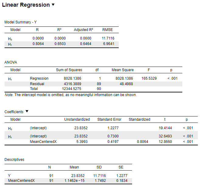
Figure 6.6: JASP Output for Regression
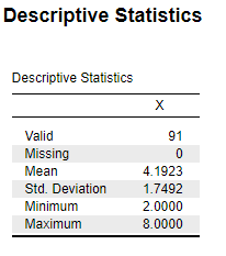
Figure 6.7: JASP Output for Descriptives
Mean-centered regression equation:
y’ = (5.3993)(x - 4.1923) + 23.8352
6.2.4 SPSS
DESCRIPTIVES VARIABLES=X
  /STATISTICS=MEAN.


REGRESSION
  /DESCRIPTIVES MEAN STDDEV CORR SIG N
  /MISSING LISTWISE
  /STATISTICS COEFF OUTS R ANOVA
  /CRITERIA=PIN(.05) POUT(.10)
  /NOORIGIN
  /DEPENDENT Y
  /METHOD=ENTER MeanCenteredX.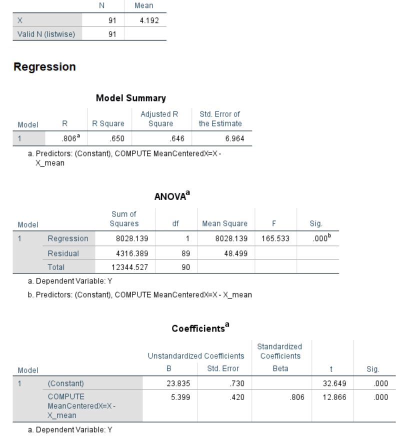
Figure 6.8: SPSS Output for Regression
Mean-centered regression equation:
y’ = (5.399)(x - 4.192) + 23.835
6.2.5 SAS
proc Reg data=Regression;
title "Linear regression";
model Y = MeanCenteredX;
run;

PROC MEANS DATA=Regression;
  VAR X Y;
RUN;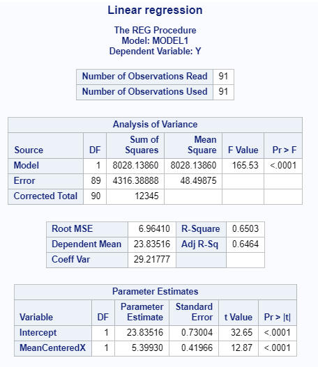
Figure 6.9: SAS Output for Regression
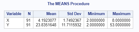
Figure 6.10: SAS Output for Means
Mean-centered regression equation:
y’ = (5.3993)(x - 4.1923077) + 23.83516
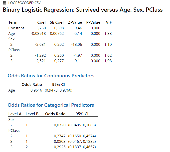
6.2.6 Minitab
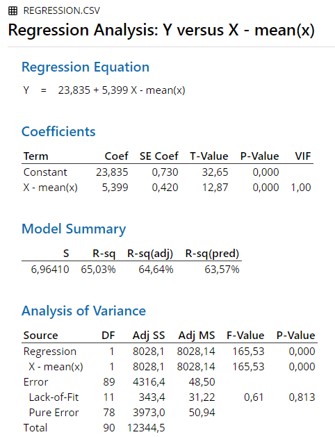
Figure 6.11: Minitab Output for Regression
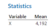
Figure 6.12: Minitab Output for Means
Mean-centered regression equation:
y’ = (5.399)(x - 4.192) + 23.835
6.2.7 R
regress.data2 <- read.csv("Datasets/Regression.csv", sep=",")
lm(formula = Y ~ MeanCenteredX, data = regress.data2)
##
## Call:
## lm(formula = Y ~ MeanCenteredX, data = regress.data2)
##
## Coefficients:
## (Intercept) MeanCenteredX
## 23.835 5.399## [1] 4.192308Mean-centered regression equation:
y’ = (5.399)(x - 4.192308) + 23.835
6.3 Logistic Regression
An example:
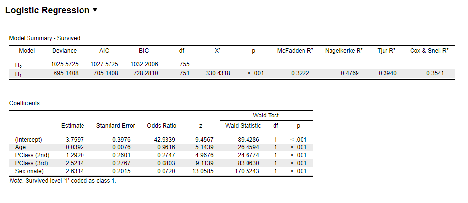
The Titanic-dataset contains original data of all passengers of the Titanic. It contains their name, their passenger class (1st - 3rd), their age, their sex, and whether or not they survived the sinking of the ship. The logistic regression model is computed to allow predictions on a passengers survival status, based on their age, sex, and passenger class.
6.3.1 Results Overview
| JASP | SPSS | SAS | Minitab | R | |
|---|---|---|---|---|---|
| Constant | 3.7597 | 3.760 | 3.7596 | 3.7600 | 3.7597 |
| Age | -0.0392 | -0.039 | -0.0392 | -0.0392 | -0.0392 |
| 2nd Class | -1.2920 | -1.292 | -1.2920 | -1.2920 | -1.2920 |
| 3rd Class | -2.5214 | -2.521 | -2.5214 | -2.5210 | -2.5214 |
| Sex(Male) | -2.6314 | -2.631 | -2.6313 | -2.6310 | -2.6314 |
| JASP | SPSS | SAS | Minitab | R | |
|---|---|---|---|---|---|
| Constant | 42.9339 | 42.934 | NA | NA | 42.9339 |
| Age | 0.9616 | 0.962 | 0.962 | 0.9616 | 0.9616 |
| 2nd Class | 0.2747 | 0.275 | 0.275 | 0.2747 | 0.2747 |
| 3rd Class | 0.0803 | 0.080 | 0.080 | 0.0803 | 0.0803 |
| Sex(Male) | 0.0720 | 0.072 | 0.072 | 0.0720 | 0.0720 |
Note: The reference case to which the odds ratios are refering is a female passenger in the first class with age 0.
6.3.3 SPSS
DATASET ACTIVATE DataSet1.
LOGISTIC REGRESSION VARIABLES Survived
  /METHOD=ENTER PClass Age Sex
  /CONTRAST (PClass)=Indicator(1)
  /CONTRAST (Sex)=Indicator(1)
  /CRITERIA=PIN(.05) POUT(.10) ITERATE(20) CUT(.5).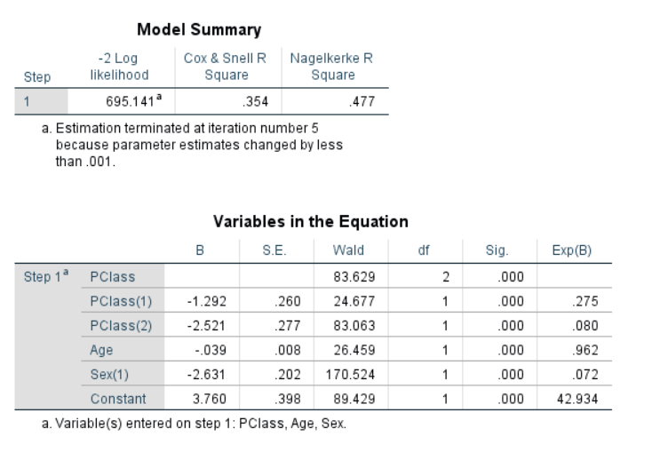
Figure 6.14: SPSS Output for Logistic Regression
6.3.4 SAS
proc logistic data=work.LogReg DESC;
  class PClass Sex / param=reference ref=first;
  model Survived = Age Sex PClass;
run;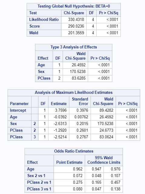
Figure 6.15: SAS Output for Logistic Regression
6.3.6 R
LogRegExample <- glm(factor(Survived) ~Age + factor(PClass) + factor(Sex), data=LogReg.data2, family=binomial(link="logit"))
summary(LogRegExample)
##
## Call:
## glm(formula = factor(Survived) ~ Age + factor(PClass) + factor(Sex),
## family = binomial(link = "logit"), data = LogReg.data2)
##
## Coefficients:
## Estimate Std. Error z value Pr(>|z|)
## (Intercept) 1.172856 0.253988 4.618 3.88e-06 ***
## Age -0.039177 0.007616 -5.144 2.69e-07 ***
## factor(PClass)1 1.271127 0.160563 7.917 2.44e-15 ***
## factor(PClass)2 -0.020835 0.138004 -0.151 0.88
## factor(Sex)1 1.315678 0.100753 13.058 < 2e-16 ***
## ---
## Signif. codes: 0 '***' 0.001 '**' 0.01 '*' 0.05 '.' 0.1 ' ' 1
##
## (Dispersion parameter for binomial family taken to be 1)
##
## Null deviance: 1025.57 on 755 degrees of freedom
## Residual deviance: 695.14 on 751 degrees of freedom
## (557 observations deleted due to missingness)
## AIC: 705.14
##
## Number of Fisher Scoring iterations: 5## (Intercept) Age factor(PClass)1 factor(PClass)2 factor(Sex)1
## 3.2312094 0.9615807 3.5648686 0.9793803 3.7272788