Chapter 8 Factor

8.1 Principal Component Analysis

An example from Field (2018 pp. 795-796):

“I have noticed that a lot of students become very stressed about SPSS Statistics. Imagine that I wanted to design a questionnaire to measure a trait that I termed ‘SPSS anxiety’. I devised a questionnaire to measure various aspects of students’ anxiety towards learning SPSS, the SAQ. I generated questions based on interviews with anxious and non-anxious students and came up with 23 possible questions to include. Each question was a statement followed by a five-point Likert scale: ‘strongly disagree’, ‘disagree’, ‘neither agree nor disagree’, ‘agree’ and ‘strongly agree’ (SD, D, N, A and SA, respectively). What’s more, I wanted to know whether anxiety about SPSS could be broken down into specific forms of anxiety. In other words, what latent variables contribute to anxiety about SPSS? With a little help from a few lecturer friends I collected 2571 completed questionnaires.”

8.1.1 Results Overview

Table 8.1: Result Overview Exploratory Factor Analysis
	JASP	SPSS	SAS	Minitab	R
SS Loading (Factor1)	3.0336	3.033	3.034	NA	3.03
SS Loading (Factor2)	2.8545	2.855	2.855	NA	2.85
SS Loading (Factor3)	1.9859	1.986	1.986	NA	1.99
SS Loading (Factor4)	1.4351	1.435	1.435	NA	1.44

8.1.2 JASP

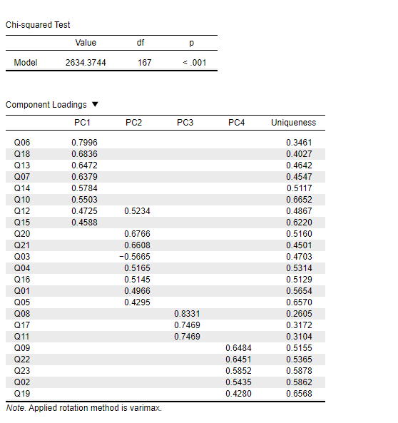
$\label{fig:pcaJASP1}JASP Output for Principal Component Analysis$

Figure 8.1: JASP Output for Principal Component Analysis

$\label{fig:pcaJASP2}JASP Output for Principal Component Analysis$

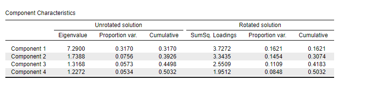
Figure 8.2: JASP Output for Principal Component Analysis

$\label{fig:pcaJASP3}JASP Output for Principal Component Analysis$

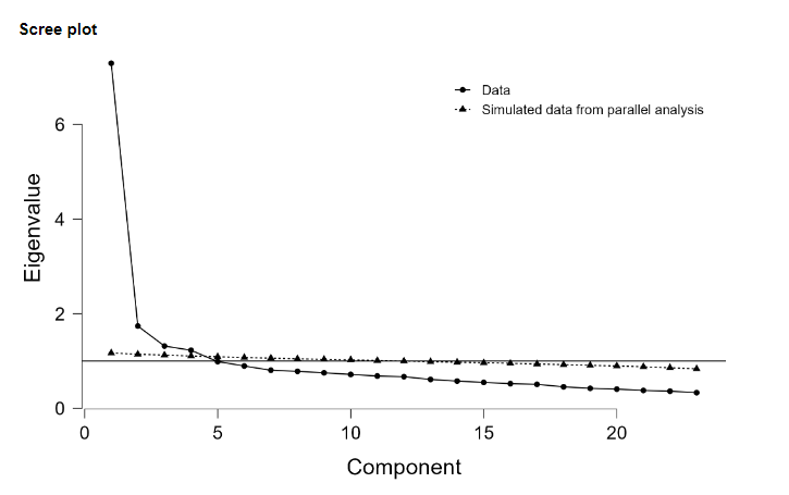
Figure 8.3: JASP Output for Principal Component Analysis

8.1.3 SPSS

DATASET ACTIVATE DataSet1.
FACTOR
  /VARIABLES Question_01 Question_02 Question_03 Question_04 Question_05 Question_06 Question_07 
    Question_08 Question_09 Question_10 Question_11 Question_12 Question_13 Question_14 Question_15 
    Question_16 Question_17 Question_18 Question_19 Question_20 Question_21 Question_22 Question_23
  /MISSING LISTWISE 
  /ANALYSIS Question_01 Question_02 Question_03 Question_04 Question_05 Question_06 Question_07 
    Question_08 Question_09 Question_10 Question_11 Question_12 Question_13 Question_14 Question_15 
    Question_16 Question_17 Question_18 Question_19 Question_20 Question_21 Question_22 Question_23
  /PRINT INITIAL ROTATION
  /PLOT EIGEN
  /CRITERIA MINEIGEN(1) ITERATE(25)
  /EXTRACTION PC
  /CRITERIA ITERATE(25)
  /ROTATION VARIMAX
  /METHOD=CORRELATION.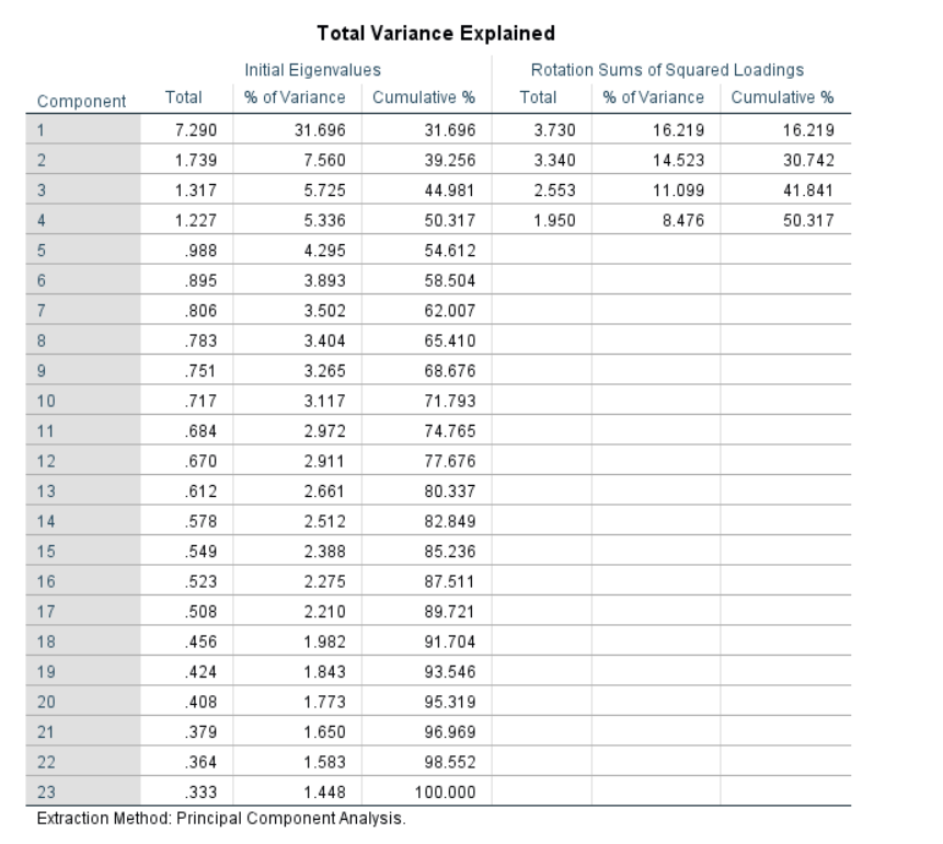

$\label{fig:pcaSPSS}SPSS Output for Principal Component Analysis$

Figure 8.4: SPSS Output for Principal Component Analysis

$\label{fig:pcaSPSS}SPSS Output for Principal Component Analysis$

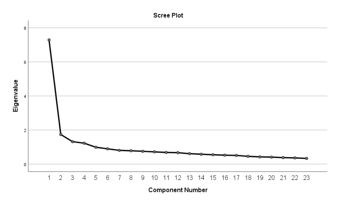
Figure 8.5: SPSS Output for Principal Component Analysis

8.1.4 SAS

PROC FACTOR Data=work.PCA scree
        Nfactors= 4
        Method= p
        Rotate=varimax;
        Var Q1 Q2 Q3 Q4 Q5 Q6 Q7 Q8 Q9 Q10 Q11 Q12 Q13 Q14 Q15 Q16 Q17 Q18 Q19 Q20 Q21 Q22 Q23
        ; 
        Run;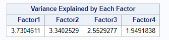

$\label{fig:pcaSAS}SAS Output for Principal Component Analysis$

Figure 8.6: SAS Output for Principal Component Analysis

$\label{fig:pcaSAS}SAS Output for Principal Component Analysis$

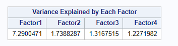
Figure 8.7: SAS Output for Principal Component Analysis

$\label{fig:pcaSAS}SAS Output for Principal Component Analysis$

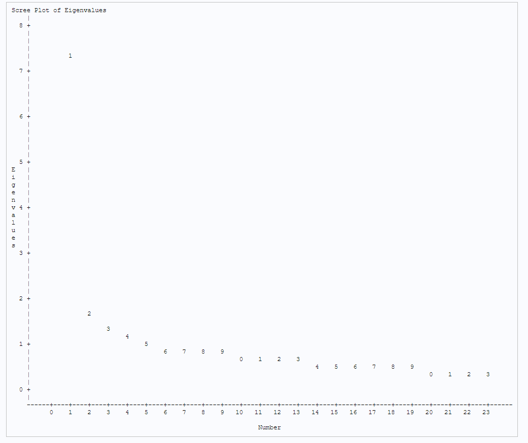
Figure 8.8: SAS Output for Principal Component Analysis

8.1.5 Minitab

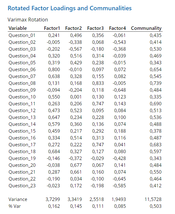
$\label{fig:pcaMinitab}Minitab Output for Principal Component Analysis$

Figure 8.9: Minitab Output for Principal Component Analysis

$\label{fig:pcaMinitab}Minitab Output for Principal Component Analysis$

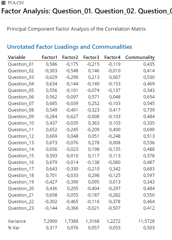
Figure 8.10: Minitab Output for Principal Component Analysis

$\label{fig:pcaMinitab}Minitab Output for Principal Component Analysis$

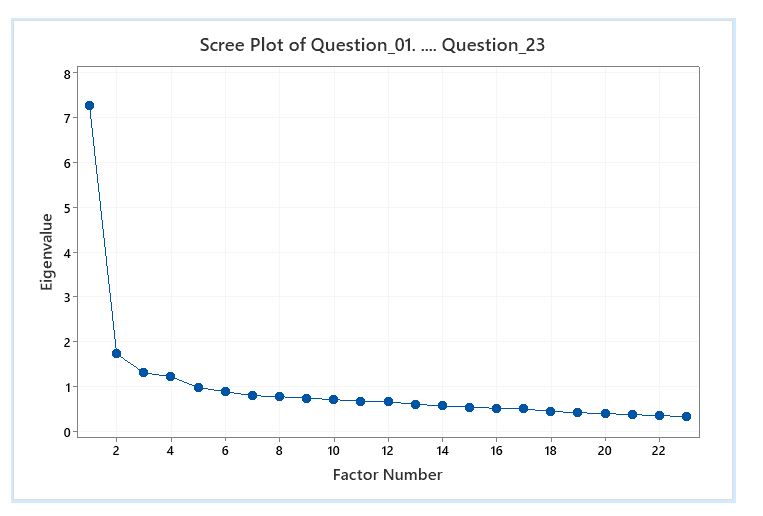
Figure 8.11: Minitab Output for Principal Component Analysis

8.1.6 R

## install.packages("psych")
## install.packages("factoextra")
## Principal Component Analysis
library("psych")

## 
## Attaching package: 'psych'

## The following object is masked from 'package:car':
## 
##     logit

library("factoextra")

## Loading required package: ggplot2

## 
## Attaching package: 'ggplot2'

## The following objects are masked from 'package:psych':
## 
##     %+%, alpha

## Welcome! Want to learn more? See two factoextra-related books at https://goo.gl/ve3WBa

fit1 <- prcomp(PCA.data, scale = TRUE) #eigenvalues
eig.val <- get_eigenvalue(fit1)
eig.val ## print results

##        eigenvalue variance.percent cumulative.variance.percent
## Dim.1   7.2900471        31.695857                    31.69586
## Dim.2   1.7388287         7.560125                    39.25598
## Dim.3   1.3167515         5.725007                    44.98099
## Dim.4   1.2271982         5.335644                    50.31663
## Dim.5   0.9878779         4.295121                    54.61175
## Dim.6   0.8953304         3.892741                    58.50449
## Dim.7   0.8055604         3.502436                    62.00693
## Dim.8   0.7828199         3.403565                    65.41050
## Dim.9   0.7509712         3.265092                    68.67559
## Dim.10  0.7169577         3.117207                    71.79280
## Dim.11  0.6835877         2.972121                    74.76492
## Dim.12  0.6695016         2.910876                    77.67579
## Dim.13  0.6119976         2.660859                    80.33665
## Dim.14  0.5777377         2.511903                    82.84855
## Dim.15  0.5491875         2.387772                    85.23633
## Dim.16  0.5231504         2.274567                    87.51089
## Dim.17  0.5083962         2.210418                    89.72131
## Dim.18  0.4559399         1.982347                    91.70366
## Dim.19  0.4238036         1.842624                    93.54628
## Dim.20  0.4077909         1.773004                    95.31929
## Dim.21  0.3794799         1.649912                    96.96920
## Dim.22  0.3640223         1.582705                    98.55191
## Dim.23  0.3330618         1.448095                   100.00000

#fviz_eig(fit1) #scree plot
fit2 <- principal(PCA.data, nfactors=4, rotate = "varimax") #varimax rotiation
fit2 ## print results

## Principal Components Analysis
## Call: principal(r = PCA.data, nfactors = 4, rotate = "varimax")
## Standardized loadings (pattern matrix) based upon correlation matrix
##               RC3   RC1   RC4   RC2   h2   u2 com
## Question_01  0.24  0.50  0.36  0.06 0.43 0.57 2.4
## Question_02 -0.01 -0.34  0.07  0.54 0.41 0.59 1.7
## Question_03 -0.20 -0.57 -0.18  0.37 0.53 0.47 2.3
## Question_04  0.32  0.52  0.31  0.04 0.47 0.53 2.4
## Question_05  0.32  0.43  0.24  0.01 0.34 0.66 2.5
## Question_06  0.80 -0.01  0.10 -0.07 0.65 0.35 1.0
## Question_07  0.64  0.33  0.16 -0.08 0.55 0.45 1.7
## Question_08  0.13  0.17  0.83  0.01 0.74 0.26 1.1
## Question_09 -0.09 -0.20  0.12  0.65 0.48 0.52 1.3
## Question_10  0.55  0.00  0.13 -0.12 0.33 0.67 1.2
## Question_11  0.26  0.21  0.75 -0.14 0.69 0.31 1.5
## Question_12  0.47  0.52  0.09 -0.08 0.51 0.49 2.1
## Question_13  0.65  0.23  0.23 -0.10 0.54 0.46 1.6
## Question_14  0.58  0.36  0.14 -0.07 0.49 0.51 1.8
## Question_15  0.46  0.22  0.29 -0.19 0.38 0.62 2.6
## Question_16  0.33  0.51  0.31 -0.12 0.49 0.51 2.6
## Question_17  0.27  0.22  0.75 -0.04 0.68 0.32 1.5
## Question_18  0.68  0.33  0.13 -0.08 0.60 0.40 1.5
## Question_19 -0.15 -0.37 -0.03  0.43 0.34 0.66 2.2
## Question_20 -0.04  0.68  0.07 -0.14 0.48 0.52 1.1
## Question_21  0.29  0.66  0.16 -0.07 0.55 0.45 1.5
## Question_22 -0.19  0.03 -0.10  0.65 0.46 0.54 1.2
## Question_23 -0.02  0.17 -0.20  0.59 0.41 0.59 1.4
## 
##                        RC3  RC1  RC4  RC2
## SS loadings           3.73 3.34 2.55 1.95
## Proportion Var        0.16 0.15 0.11 0.08
## Cumulative Var        0.16 0.31 0.42 0.50
## Proportion Explained  0.32 0.29 0.22 0.17
## Cumulative Proportion 0.32 0.61 0.83 1.00
## 
## Mean item complexity =  1.8
## Test of the hypothesis that 4 components are sufficient.
## 
## The root mean square of the residuals (RMSR) is  0.06 
##  with the empirical chi square  4006.15  with prob <  0 
## 
## Fit based upon off diagonal values = 0.96

8.1.7 Remarks

The rotation used was “Varimax”. The differences in the results of the rotated factor solutions between the software are due to differences in the optimization methods used.

8.1.8 References

Field, A. (2018). Discovering statistics using IBM SPSS statistics. Los Angeles, CA: SAGE.

8.2 Exploratory Factor Analysis

An example from Field (2018 pp. 795-796):

8.2.1 Results Overview

Table 8.2: Result Overview Exploratory Factor Analysis
	JASP	SPSS	SAS	Minitab	R
SS Loading (Factor1)	3.0336	3.033	3.034	NA	3.03
SS Loading (Factor2)	2.8545	2.855	2.855	NA	2.85
SS Loading (Factor3)	1.9859	1.986	1.986	NA	1.99
SS Loading (Factor4)	1.4351	1.435	1.435	NA	1.44

8.2.2 JASP

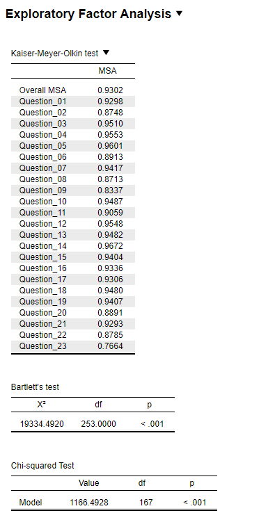
$\label{fig:efaJASP}JASP Output for Exploratory Factor Analysis$

Figure 8.12: JASP Output for Exploratory Factor Analysis

$\label{fig:efaJASP2}JASP Output for Exploratory Factor Analysis$

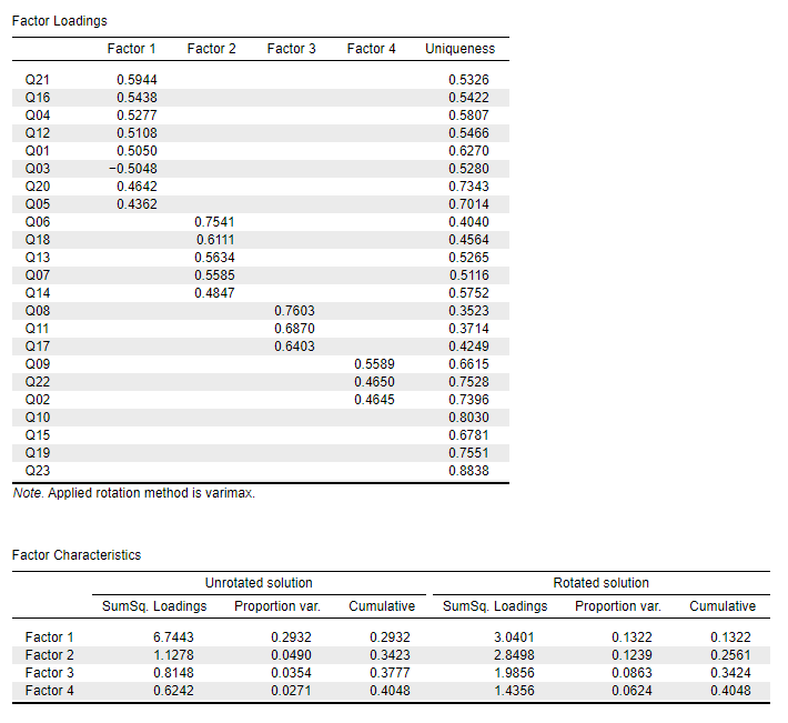
Figure 8.13: JASP Output for Exploratory Factor Analysis

$\label{fig:efaJASP3}JASP Output for Exploratory Factor Analysis$

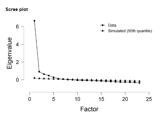
Figure 8.14: JASP Output for Exploratory Factor Analysis

8.2.3 SPSS

FACTOR
  /VARIABLES Question_01 Question_02 Question_03 Question_04 Question_05 Question_06 Question_07 
    Question_08 Question_09 Question_10 Question_11 Question_12 Question_13 Question_14 Question_15 
    Question_16 Question_17 Question_18 Question_19 Question_20 Question_21 Question_22 Question_23
  /MISSING LISTWISE 
  /ANALYSIS Question_01 Question_02 Question_03 Question_04 Question_05 Question_06 Question_07 
    Question_08 Question_09 Question_10 Question_11 Question_12 Question_13 Question_14 Question_15 
    Question_16 Question_17 Question_18 Question_19 Question_20 Question_21 Question_22 Question_23
  /PRINT INITIAL KMO EXTRACTION ROTATION
  /CRITERIA MINEIGEN(1) ITERATE(25)
  /EXTRACTION PAF
  /CRITERIA ITERATE(25)
  /ROTATION VARIMAX
  /METHOD=CORRELATION.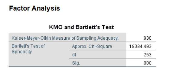

$\label{fig:efaSPSS}SPSS Output for Exploratory Factor Analysis$

Figure 8.15: SPSS Output for Exploratory Factor Analysis

$\label{fig:efaSPSS2}SPSS Output for Exploratory Factor Analysis$

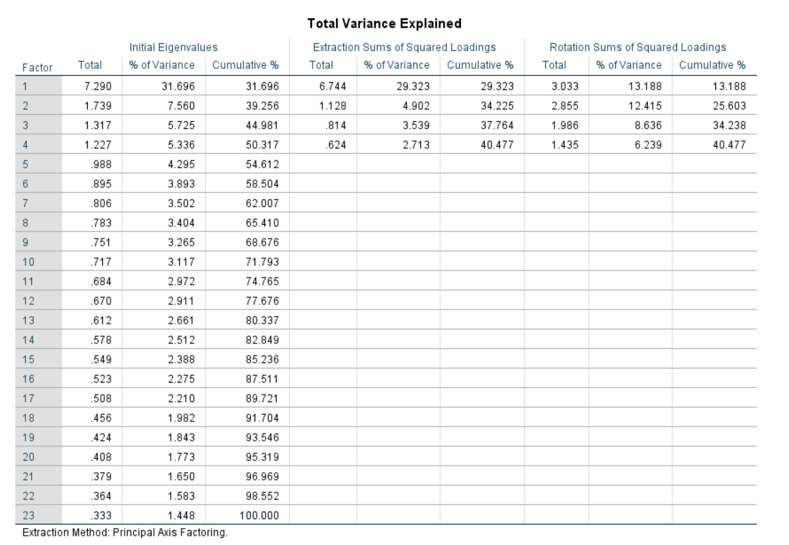
Figure 8.16: SPSS Output for Exploratory Factor Analysis

8.2.4 SAS

PROC FACTOR Data=work.efa scree
        Nfactors= 4
        Method= prinit
        Rotate=varimax;
        Var Q1 Q2 Q3 Q4 Q5 Q6 Q7 Q8 Q9 Q10 Q11 Q12 Q13 Q14 Q15 Q16 Q17 Q18 Q19 Q20 Q21 Q22 Q23
        ; 
        Run;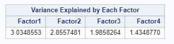

$\label{fig:efaSAS}SAS Output for Exploratory Factor Analysis$

Figure 8.17: SAS Output for Exploratory Factor Analysis

$\label{fig:efaSAS2}SAS Output for Exploratory Factor Analysis$

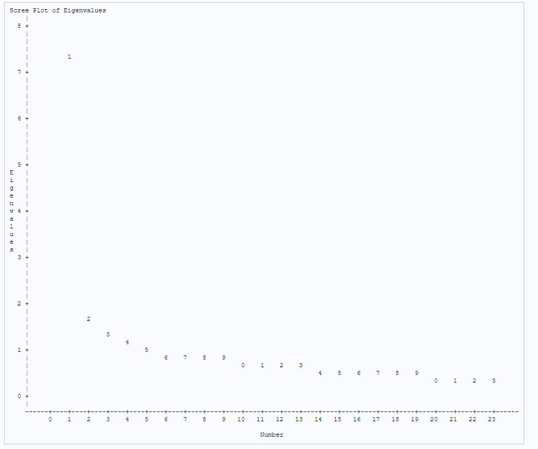
Figure 8.18: SAS Output for Exploratory Factor Analysis

8.2.5 Minitab

Exploratory Factor Analysis with Principal Axis Factoring is not available in Minitab.

8.2.6 R

## install.packages("psych")
## Principal Axis Factor Analysis
library("psych")
fit <- factor.pa(EFA.data, nfactors=4, rotate = "varimax")

## Warning: factor.pa is deprecated. Please use the fa function with fm=pa

fit ## print results

## Factor Analysis using method =  pa
## Call: factor.pa(r = EFA.data, nfactors = 4, rotate = "varimax")
## Unstandardized loadings (pattern matrix) based upon covariance matrix
##               PA1   PA3   PA4   PA2   h2   u2   H2   U2
## Question_01  0.50  0.22 -0.27  0.00 0.37 0.63 0.37 0.63
## Question_02 -0.21 -0.03 -0.01  0.46 0.26 0.74 0.26 0.74
## Question_03 -0.50 -0.18  0.16  0.40 0.47 0.53 0.47 0.53
## Question_04  0.53  0.28 -0.25 -0.03 0.42 0.58 0.42 0.58
## Question_05  0.44  0.27 -0.19 -0.05 0.30 0.70 0.30 0.70
## Question_06  0.05  0.75 -0.12 -0.10 0.59 0.41 0.59 0.41
## Question_07  0.36  0.56 -0.16 -0.13 0.49 0.51 0.49 0.51
## Question_08  0.22  0.15 -0.76  0.00 0.65 0.35 0.65 0.35
## Question_09 -0.13 -0.07 -0.06  0.56 0.34 0.66 0.34 0.66
## Question_10  0.14  0.38 -0.14 -0.12 0.20 0.80 0.20 0.80
## Question_11  0.24  0.27 -0.69 -0.17 0.63 0.37 0.63 0.37
## Question_12  0.51  0.40 -0.11 -0.15 0.45 0.55 0.45 0.55
## Question_13  0.29  0.56 -0.23 -0.14 0.47 0.53 0.47 0.53
## Question_14  0.39  0.49 -0.15 -0.13 0.42 0.58 0.42 0.58
## Question_15  0.28  0.38 -0.25 -0.20 0.32 0.68 0.32 0.68
## Question_16  0.54  0.28 -0.25 -0.16 0.46 0.54 0.46 0.54
## Question_17  0.29  0.27 -0.64 -0.05 0.58 0.42 0.58 0.42
## Question_18  0.37  0.61 -0.14 -0.13 0.54 0.46 0.54 0.46
## Question_19 -0.28 -0.15  0.06  0.38 0.24 0.76 0.24 0.76
## Question_20  0.46  0.04 -0.09 -0.20 0.27 0.73 0.27 0.73
## Question_21  0.59  0.26 -0.15 -0.15 0.47 0.53 0.47 0.53
## Question_22 -0.03 -0.16  0.07  0.47 0.25 0.75 0.25 0.75
## Question_23  0.03 -0.04  0.07  0.33 0.12 0.88 0.12 0.88
## 
##                        PA1  PA3  PA4  PA2
## SS loadings           3.03 2.85 1.99 1.44
## Proportion Var        0.13 0.12 0.09 0.06
## Cumulative Var        0.13 0.26 0.34 0.40
## Proportion Explained  0.33 0.31 0.21 0.15
## Cumulative Proportion 0.33 0.63 0.85 1.00
## 
##  Standardized loadings (pattern matrix)
##             item   PA1   PA3   PA4   PA2   h2   u2
## Question_01    1  0.50  0.22 -0.27  0.00 0.37 0.63
## Question_02    2 -0.21 -0.03 -0.01  0.46 0.26 0.74
## Question_03    3 -0.50 -0.18  0.16  0.40 0.47 0.53
## Question_04    4  0.53  0.28 -0.25 -0.03 0.42 0.58
## Question_05    5  0.44  0.27 -0.19 -0.05 0.30 0.70
## Question_06    6  0.05  0.75 -0.12 -0.10 0.59 0.41
## Question_07    7  0.36  0.56 -0.16 -0.13 0.49 0.51
## Question_08    8  0.22  0.15 -0.76  0.00 0.65 0.35
## Question_09    9 -0.13 -0.07 -0.06  0.56 0.34 0.66
## Question_10   10  0.14  0.38 -0.14 -0.12 0.20 0.80
## Question_11   11  0.24  0.27 -0.69 -0.17 0.63 0.37
## Question_12   12  0.51  0.40 -0.11 -0.15 0.45 0.55
## Question_13   13  0.29  0.56 -0.23 -0.14 0.47 0.53
## Question_14   14  0.39  0.48 -0.15 -0.13 0.42 0.58
## Question_15   15  0.28  0.38 -0.25 -0.20 0.32 0.68
## Question_16   16  0.54  0.28 -0.25 -0.16 0.46 0.54
## Question_17   17  0.30  0.27 -0.64 -0.05 0.58 0.42
## Question_18   18  0.37  0.61 -0.14 -0.13 0.54 0.46
## Question_19   19 -0.28 -0.15  0.06  0.37 0.24 0.76
## Question_20   20  0.47  0.04 -0.09 -0.20 0.27 0.73
## Question_21   21  0.60  0.26 -0.15 -0.15 0.47 0.53
## Question_22   22 -0.03 -0.16  0.07  0.47 0.25 0.75
## Question_23   23  0.03 -0.04  0.07  0.33 0.12 0.88
## 
##                  PA1  PA3  PA4  PA2
## SS loadings     3.03 2.85 1.99 1.44
## Proportion Var  0.13 0.12 0.09 0.06
## Cumulative Var  0.13 0.26 0.34 0.40
## Cum. factor Var 0.33 0.63 0.85 1.00
## 
## Mean item complexity =  1.8
## Test of the hypothesis that 4 factors are sufficient.
## 
## The degrees of freedom for the null model are  253  and the objective function was  7.55 with Chi Square of  19334.49
## The degrees of freedom for the model are 167  and the objective function was  0.46 
## 
## The root mean square of the residuals (RMSR) is  0.03 
## The df corrected root mean square of the residuals is  0.03 
## 
## The harmonic number of observations is  2571 with the empirical chi square  880.48  with prob <  2.3e-97 
## The total number of observations was  2571  with Likelihood Chi Square =  1166.49  with prob <  2.1e-149 
## 
## Tucker Lewis Index of factoring reliability =  0.921
## RMSEA index =  0.048  and the 90 % confidence intervals are  0.046 0.051
## BIC =  -144.8
## Fit based upon off diagonal values = 0.99
## Measures of factor score adequacy             
##                                                    PA1  PA3  PA4  PA2
## Correlation of (regression) scores with factors   0.83 0.86 0.86 0.77
## Multiple R square of scores with factors          0.69 0.73 0.74 0.59
## Minimum correlation of possible factor scores     0.37 0.46 0.49 0.19

8.2.7 Remarks

The method used was “Principal Axis Factoring” and the rotation used was “Varimax”. The differences in the results of the rotated factor solutions between the software are due to differences in the optimization methods used.

8.2.8 References

Field, A. (2018). Discovering statistics using IBM SPSS statistics. Los Angeles, CA: SAGE.