Chapter 3 T-Tests
3.1 Independent Samples T-Test
An example from Hays (1974, pp. 404-407):
“An experimenter working in the area of motivational factors in perception was interested in the effects of deprivation upon the perceived size of objects. Among the studies carried out was one done with orphans, who were compared with nonorphaned children on the basis of the judged size of parental figures viewed at a distance. […]Now two independent randomly selected groups were used. Sample 1 was a group of orphaned children without foster parents. Sample 2 was a group of children having a normal family with both parents. Both population of children sampled showed the same age level, sex distribution, educational level, and so forth. The question asked by the experimenter was ‘Do deprived children tend to judge the parental figures relatively larger than do the nondeprived?’ In terms of a null and alternative hypothesis,
H0: \(\mu\)1 - \(\mu\)2 \(\le 0\)
H1: \(\mu\)1 - \(\mu\)2 \(> 0\).
The \(\alpha\) level for significance decided upon was .05. The actual results were
Sample 1:
M1 = 1.8
S1 = .7
N1 = 125
Sample 2:
M2 = 1.6
S2 = .9
N2 = 150”
Note: A data set with these properties has been simulated using R.
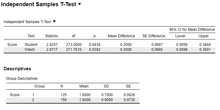
3.1.1 Results Overview
| By Hand | JASP | SPSS | SAS | Minitab | R | |
|---|---|---|---|---|---|---|
| t (Welch) | 2.11 | 2.0717 | 2.072 | 2.07 | 2.07 | 2.0717 |
| t (Student) | NA | 2.0257 | 2.026 | 2.03 | 2.03 | 2.0257 |
3.1.2 By Hand
Calculations by hand can be found in Hays, 1974, pp. 404-407.
Result: t = 2.11
Significant (two-tailed test) for \(\alpha\) = .05 or less
Note: Hays calculated only the Welch T-test.
3.1.4 SPSS
DATASET ACTIVATE DataSet1.
T-TEST GROUPS=groups(1 2)
  /MISSING=ANALYSIS
  /VARIABLES=samples
  /CRITERIA=CI(.95).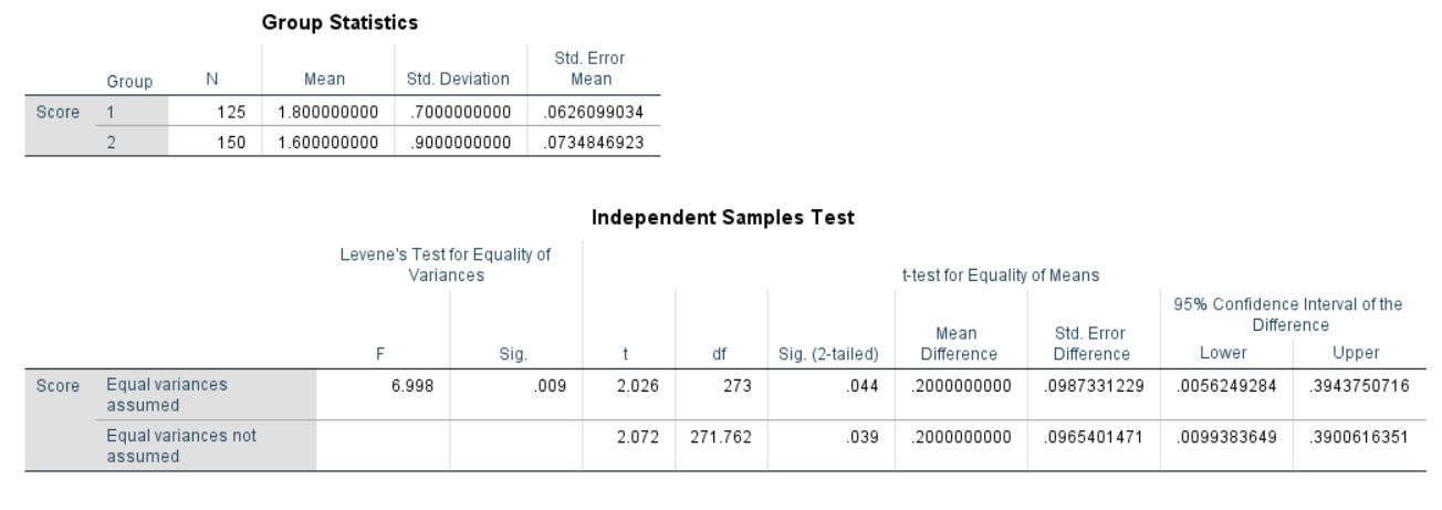
Figure 3.2: SPSS Output for Independent Samples T-Test
3.1.5 SAS
proc ttest data=istt sides=2 alpha=0.05 h0=0;
    title "Two sample t-test";
    class Group;
    var Score;
   run;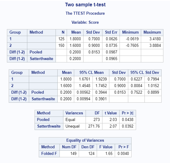
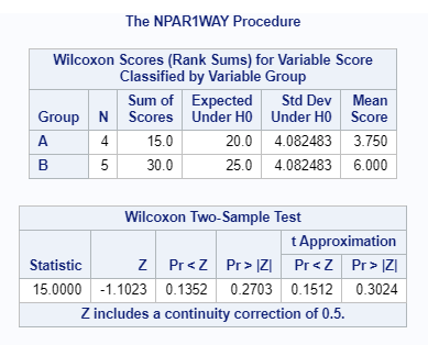
Figure 3.3: SAS Output for Independent Samples T-Test
3.1.6 Minitab
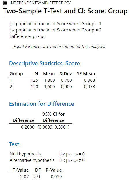
Figure 3.4: Minitab Output for Welch Independent Samples T-Test
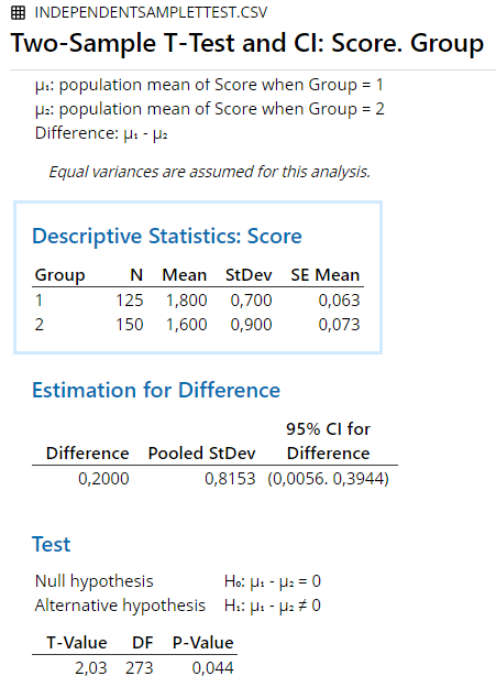
Figure 3.5: Minitab Output for Student Independent Samples T-Test
3.1.7 R
##
##  Welch Two Sample t-test
##
## data:  subset(istt.data, Group == 1)$Score and subset(istt.data, Group == 2)$Score
## t = 2.0717, df = 271.76, p-value = 0.03924
## alternative hypothesis: true difference in means is not equal to 0
## 95 percent confidence interval:
##  0.009938365 0.390061635
## sample estimates:
## mean of x mean of y
## 1.8 1.6##
## Two Sample t-test
##
## data: subset(istt.data, Group == 1)$Score and subset(istt.data, Group == 2)$Score
## t = 2.0257, df = 273, p-value = 0.04377
## alternative hypothesis: true difference in means is not equal to 0
## 95 percent confidence interval:
## 0.005624928 0.394375072
## sample estimates:
## mean of x mean of y
## 1.8 1.63.2 Mann-Whitney Test
An example from Hays (1974, pp. 778-780):
“As an example, consider the following data:”
| Score | Group |
|---|---|
| 8 | A |
| 3 | A |
| 4 | A |
| 6 | A |
| 1 | B |
| 7 | B |
| 9 | B |
| 10 | B |
| 12 | B |
3.2.1 Results Overview
| By Hand | JASP | SPSS | SAS | Minitab | R | |
|---|---|---|---|---|---|---|
| U’ | 5 | 5 | 5 | 5 | 5 | 5 |
3.2.2 By Hand
Calculations by hand can be found in Hays, 1974, pp. 778-780.
Result:
U’ = 5
U = 15
Not significant for \(\alpha\) = .05 or less.
3.2.3 JASP
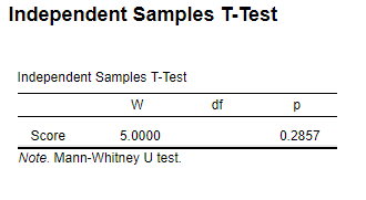
Figure 3.6: JASP Output for Mann-Whitney Test
Note: W corresponds to U’ in the hand calculation.
3.2.4 SPSS
DATASET ACTIVATE DataSet1.
*Nonparametric Tests: Independent Samples.
NPTESTS
  /INDEPENDENT TEST (Score) GROUP (Group) MANN_WHITNEY
  /MISSING SCOPE=ANALYSIS USERMISSING=EXCLUDE
  /CRITERIA ALPHA=0.05  CILEVEL=95.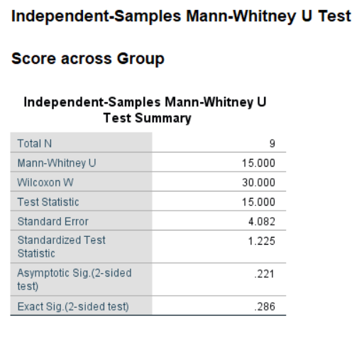
Figure 3.7: SPSS Output for Mann-Whitney Test
Note: U = 15 corresponds to U’ = 5.
3.2.6 Minitab
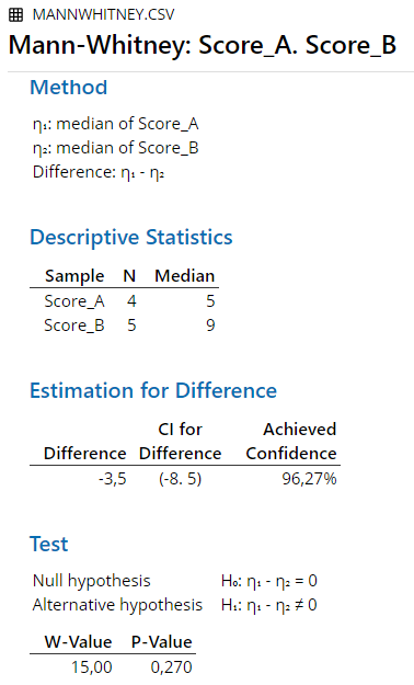
Figure 3.9: Minitab Output for Mann-Whitney Test
Note: W corresponds to U in the hand calculation and U = 15 corresponds to U’ = 5.
3.2.7 R
##
##  Wilcoxon rank sum exact test
##
## data:  Score by Group
## W = 5, p-value = 0.2857
## alternative hypothesis: true location shift is not equal to 0
Note: W corresponds to U’ in the hand calculation.
3.2.8 Remarks
All differences in results between the software and hand calculation are due to rounding.
The output for the Mann-Whitney test is not clearly defined, leading to different conventions in different software. The R documentation explains it as follows:
“The two most common definitions correspond to the sum of the ranks of the first sample with the minimum value subtracted or not: R subtracts and S-PLUS does not, giving a value which is larger by m(m+1)/2 for a first sample of size m. (It seems Wilcoxon’s original paper used the unadjusted sum of the ranks but subsequent tables subtracted the minimum.) R’s value can also be computed as the number of all pairs (x[i], y[j]) for which y[j] is not greater than x[i], the most common definition of the Mann-Whitney test.”
3.3 Paired Samples T-Test
An example from Hays (1974, pp. 424-427):
“Consider once again the question of scores on a test of dominance. The basic question has to do with the mean score for men as opposed to the mean score for women. In carrying out the experiment, the investigator decided to sample eight husband-wife-pairs at random. The members of each pair were given the test of dominance separately, and the data turned out as follows:”
| Husband | Wife |
|---|---|
| 26 | 30 |
| 28 | 29 |
| 28 | 28 |
| 29 | 27 |
| 30 | 26 |
| 31 | 25 |
| 34 | 24 |
| 37 | 23 |
3.3.1 Results Overview
| By Hand | JASP | SPSS | SAS | Minitab | R | |
|---|---|---|---|---|---|---|
| t | 1.838 | 1.8381 | 1.838 | 1.84 | 1.84 | 1.8381 |
3.3.2 By Hand
Calculations by hand can be found in Hays, 1974, pp. 424-427.
Result: t = 1.838
Not significant (two-tailed test) for \(\alpha\) = .05 or less.
3.3.4 SPSS
DATASET ACTIVATE DataSet1.
T-TEST PAIRS=Husband WITH Wife (PAIRED)
  /CRITERIA=CI(.9500)
  /MISSING=ANALYSIS.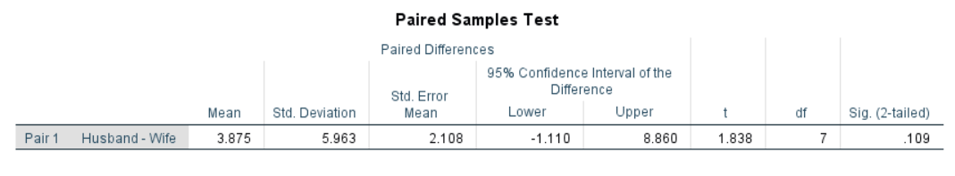
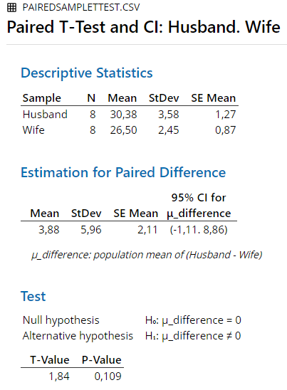
Figure 3.11: SPSS Output for Paired Samples T-Test
3.3.5 SAS
proc ttest data=pstt sides=2 alpha=0.05 h0=0;
title "Paired sample t-test";
paired Husband * Wife;
run;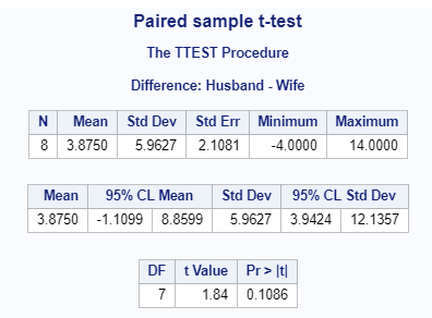
Figure 3.12: SAS Output for Paired Samples T-Test
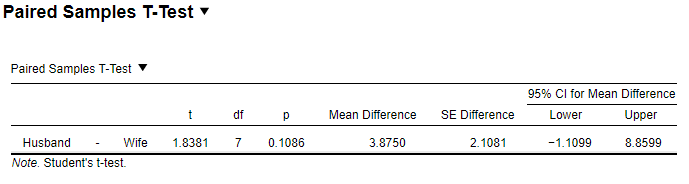
3.3.7 R
##
##  Paired t-test
##
## data:  pstt.data$Husband and pstt.data$Wife
## t = 1.8381, df = 7, p-value = 0.1086
## alternative hypothesis: true mean difference is not equal to 0
## 95 percent confidence interval:
##  -1.109927  8.859927
## sample estimates:
## mean difference
## 3.8753.4 Wilcoxon Test
An example from Hays (1974, pp. 780-781):
“Suppose that in some experiment involving a single treatment and one control group, subjects were first matched pairwise, and then one member of each pair was assigned to the experimental group at random. In the experiment proper, each subject received some Y score.”
| Treatment. | Control |
|---|---|
| 83 | 75 |
| 80 | 78 |
| 81 | 66 |
| 74 | 77 |
| 79 | 80 |
| 78 | 68 |
| 72 | 75 |
| 84 | 90 |
| 85 | 81 |
| 88 | 83 |
3.4.1 Results Overview
| By Hand | JASP | SPSS | SAS | Minitab | R | |
|---|---|---|---|---|---|---|
| W’ | 15 | 15 | 15 | NA | 15 | 15 |
3.4.2 By Hand
Calculations by hand can be found in Hays, 1974, pp. 780-781.
Result:
T = 15
Not significant for \(\alpha\) = .05 or less.
3.4.4 SPSS
DATASET ACTIVATE DataSet1.
*Nonparametric Tests: Related Samples.
NPTESTS
/RELATED TEST(Treatment Control) WILCOXON
/MISSING SCOPE=ANALYSIS USERMISSING=EXCLUDE
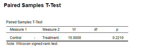
/CRITERIA ALPHA=0.05 CILEVEL=95.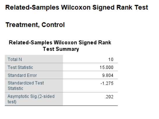
Figure 3.15: SPSS Output for Wilcoxon Test
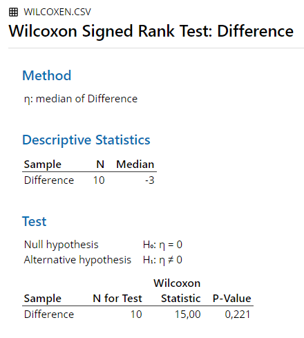
3.4.7 R
## Warning in wilcox.test.default(Wilcoxon.data2$Control,
## Wilcoxon.data2$Treatment., : cannot compute exact p-value with ties
##
## Wilcoxon signed rank test with continuity correction
##
## data: Wilcoxon.data2$Control and Wilcoxon.data2$Treatment.
## V = 15, p-value = 0.221
## alternative hypothesis: true location shift is not equal to 03.5 One Sample T-Test
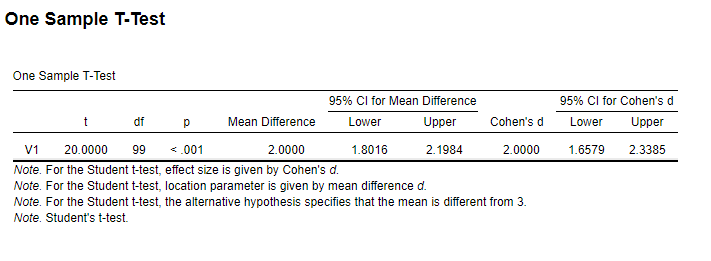
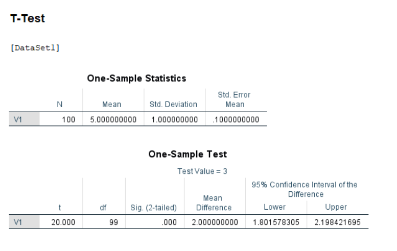
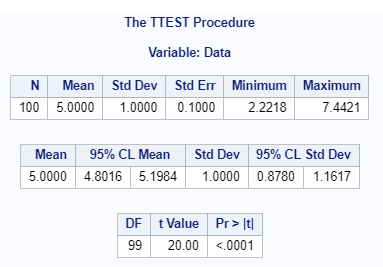
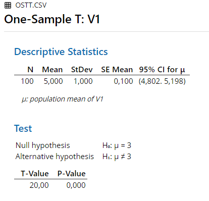
A dataset with the following properties has been generated using R:
n = 100
M = 5
\(\sigma\) = 1
The expected mean to perform the One Sample T-test against is:
E(M) = 3
The alpha level was chosen to be:
\(\alpha\) = .05
3.5.1 Results Overview
| By Hand | JASP | SPSS | SAS | Minitab | R | |
|---|---|---|---|---|---|---|
| t | 20 | 20 | 20 | 20 | 20 | 20 |
3.5.2 By Hand
t = \(\frac{M - E(M) }{\sigma/\sqrt{n}}\)
therefore:
t = \(\frac{5-3}{1/\sqrt{100}}\) = \(\frac{2}{1/10}\) = 20
A t-score of 20 is significant for a two tailed test at \(\alpha\) = .05 or less.